SimCLR Multi GPU with Tensorflow
In recent years, self-supervised learning for computer vision has transitioned from pretext tasks to siamese based representation learning. One popular method is SimCLR, in which the model tries to learn a representation of the data, which is agnostic to augmentations. The authors found that to achieve the best performance, they had to train with (very) large batch sizes such as 8192! Training with large batch sizes on (224x224x3) images forces us to distribute the training to multiple GPUs. Trivially splitting the batch into smaller chunks and distributing the chunks across GPUs won’t work (I mean, it will work, but it is wrong :) ). I’ll get into the details later, but in short, the SimCLR loss compares each image with all other images in the batch, and if the batch is split into chunks, each GPU will compare each image only to other images in its chunk.
In this post, I will explain how to implement SimCLR loss on a single GPU with tensorflow and then modify the code to be correct in a distributed environment. I assume you have some knowledge of contrastive models and basic tensorflow.
SimCLR (tiny) Introduction
SimCLR learns image representations by making the output embedding between differently augmented views of the same image close in the latent space and distant between views of different images.
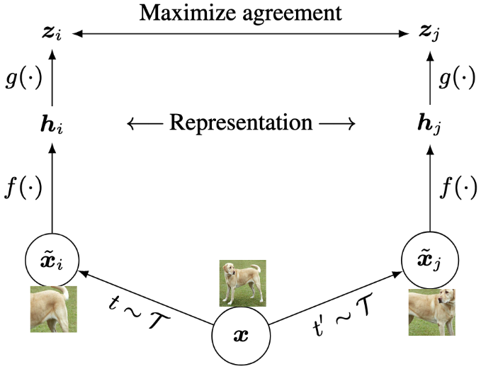
As illustrated in the figure, these are the major framework components.
- Stochastic data augmentation - transforms any input image \(x\) to two correlated views of the same image denoted \(\tilde{x_i}\) \(\tilde{x_j}\).
- Neural network backbone/encoder f(⋅) - extracts a representation/embedding vector for each augmented view. This is the network being pre-trained and used in some downstream tasks. I use a resnet-50 in this post.
- Small MLP projection head \(g(\cdot)\) that maps representations to the space where contrastive loss is applied.
- Contrastve loss function. Forces different views of the same image to have similar embeddings, while embeddings of views from different images to be dissimilar.
NT-Xent Contrastive Loss
Every input image in a batch of size N goes through two random series of augmentations that pass through \(f(\cdot)\) and \(g(\cdot)\), creating \(N\) positive embedding pairs \(z_i\) \(z_j\). Given a positive pair, all the other \(2(N-1)\) augmented examples within the batch are considered negative examples. Let \(sim(z_i,z_j)\) be the cosine similarity between \(z_i\) and \(z_j\) divided by some temperature hyperparameter \(\tau\), and \(\mathbb I_{[k\neq i]}\) an indicator function evaluating to 1 iff \(k\neq i.\) Then, the loss for a positive pair \((i,j)\) is defined as
\[l_{i,j}= -log { e^{sim(z_i,z_j)} \over \sum_{k=1}^{2N} \mathbb I_{[k\neq i]} e^{sim(z_i,z_k)} } \]
While training, the optimizer will minimize the loss function, forcing \(sim(z_i,z_j)\) to be as big as possible for each positive pair \(i,j\) and as small as possible for every negative pair.
Single GPU Loss Implementation
The result of a batch of N images being augmented and passed through \(g(f(\cdot))\) is two tensors hidden1 and hidden2. hidden1 and hidden2 contain the \(z_i\) ,\(z_j\) tensors, respectfully. The shape of these tensors is \((N,dim)\) - \(N\) being the batch size and \(dim\) being the dimension of the \(z\) embedding:
Using hidden1 and hidden2, I can compute the loss \(l_{i,j}\) for every couple in the batch at once.
First, I compute \(sim(x,y)\) between every \(z_i\) in hidden1 and every \(z_j\) in hidden2 and store the results in logits_ab
hidden1 = tf.math.l2_normalize(hidden1, -1)
hidden2 = tf.math.l2_normalize(hidden2, -1)
logits_ab = tf.matmul(hidden1, hidden2, transpose_b=True) / self.temperature
Next, compute \(sim(x,y)\) between every \(z_i\) in hidden1 and every other \(z_i\) in hidden1 and store the results in logits_aa
logits_aa = tf.matmul(hidden1, hidden1, transpose_b=True) / self.temperature
logits_aa and logits_ab are both symmetric tensors shaped \(N\times N\), where logits_ab[x,y] contains the \(sim\) between hidden1[x] and hidden2[y] and logits_aa[x,y] contains the \(sim\) between hidden1[x] and hidden1[y]. The diagonal of hidden_ab contains the \(sim\) between the positive pairs, and the diagonal of hidden_aa contains the \(sim\) between every \(z_i\) and itself.
Concatenating logits_ab with logits_aa creates a new matrix called logits:
logits = tf.concat([logits_ab, logits_aa], 1)
Lets examine a single row \(k\) in logits:
\(\color{blue}{ab_{k,k}}\) is the \(sim\) between the positive \(k\) pair, which is the value we want to increase in the loss dominator. \(\color{red}{aa_{k,k}}\) is the \(sim\) between hidden[k] and itself, which is the value we want to ignore using the indicator function \(\mathbb I_{[k\neq i]}\).
To ignore \(\color{red}{aa_{k,k}}\) in the later calculation, I replace it with a small number before creating logits (this will be clearer later):
masks = tf.one_hot(tf.range(batch_size), batch_size)
logits_aa = logits_aa - masks * 1e9 # substract large number from diagonal
Finally, to calculate the loss on a single pair \(z_i\) \(z_j\), represented by row \(k\) of logits, we calculate softmax_cross_entropy_with_logits between row \(k\) and a label tensor consisting of \(0\) except for \(1\) at index \(k\). softmax_cross_entropy_with_logits will first calculate the softmax of the row producing the \(e^{sim} \over \sum_{k=1}^{2N} \mathbb I_{[k\neq i]} e^{sim}\) term for each index. Next, the function will calculate the cross entropy, but because label is \(1\) only at index \(k\), the whole row is discarded except for index \(k\) which gives us precisely the \(l_{i,j}\) loss.
The small number we manually put in \(\color{red}{aa_{k,k}}\) will cause the exponent to become \(0\), which implements our indicator function.
labels = tf.one_hot(tf.range(batch_size), batch_size * 2) # 1 at index k for each row
loss = tf.nn.softmax_cross_entropy_with_logits(labels, logits, 1))
The final loss function:
class SimCLRLoss(tf.keras.losses.Loss):
    LARGE_NUM = 1e9

    def __init__(self, temperature: float = 0.05, **kwargs):

        super().__init__(**kwargs)
        self.temperature = temperature

    def contrast(self, hidden1, hidden2):

        batch_size = tf.shape(hidden1)[0]

        labels = tf.one_hot(tf.range(batch_size), batch_size * 2)
        masks = tf.one_hot(tf.range(batch_size), batch_size)

        logits_aa = tf.matmul(hidden1, hidden1, transpose_b=True) / self.temperature
        logits_aa = logits_aa - masks * SimCLRLoss.LARGE_NUM

        logits_ab = tf.matmul(hidden1, hidden2, transpose_b=True) / self.temperature
        loss_a = tf.nn.softmax_cross_entropy_with_logits(labels, tf.concat([logits_ab, logits_aa], 1))

        return loss_a

    def call(self, hidden1, hidden2):
        hidden1 = tf.math.l2_normalize(hidden1, -1)
        hidden2 = tf.math.l2_normalize(hidden2, -1)
        loss_a = self.contrast(hidden1, hidden2)
        loss_b = self.contrast(hidden2, hidden1) # called second time to compute L(zj,zi)

        return loss_a + loss_b
Multi GPU Loss Implementation
SimCLR loss is special compared to other loss functions because the loss for a single sample is computed using other samples in the batch instead of just itself. This requires some changes to our loss implementation.
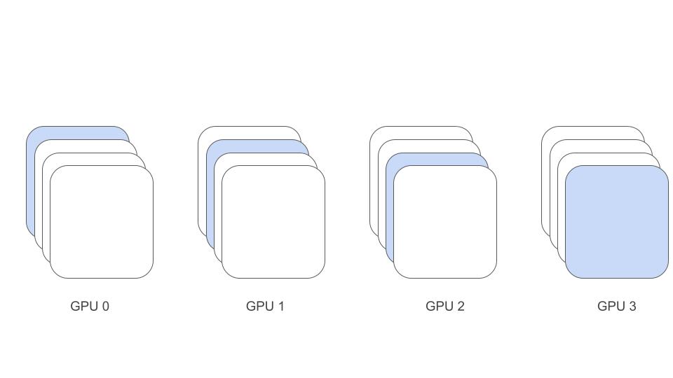
When using multiple GPUs with a distributed strategy, tensorflow will split the batch into smaller batches and distribute each small batch to a different GPU.
Using the loss implementation from before in a distributed strategy will work! Batches will be distributed, losses will be calculated, parameters will be updated, and metrics will improve! However, nothing will be working correctly!
In the SimCLR paper, the authors show that their framework benefits from larger batch sizes. Larger batch sizes provide more negative examples for each positive pair, so the denominator in the loss \(l_{i,j}\) contains more negative couples. If we take our large batch of 8192 and naively distribute it across 8 GPUs, each GPU will calculate the contrastive loss on 1024 examples, so each positive pair will only be compared against the other 1023 pairs and not all the other 8191 pairs in the global batch.
We want to enjoy both worlds, distribute the batch to multiple GPUs, and compare each pair with ALL other pairs across GPUs.
This is done by constructing the \(logits\) matrix from before a bit differently.
First, sync all GPUs to create the large hidden1 and hidden2 containing embeddings of all global_batch_size images:
ext_tensor = tf.scatter_nd(
    indices=[[replica_context.replica_id_in_sync_group]],
    updates=[hidden],
    shape=tf.concat([[num_replicas], tf.shape(hidden)], axis=0),
)
ext_tensor = replica_context.all_reduce(tf.distribute.ReduceOp.SUM, ext_tensor)
hidden_large =  tf.reshape(ext_tensor, [-1] + ext_tensor.shape.as_list()[2:])
The scatter_nd will run on each GPU and take the per_batch hidden and place it in ext_tensor. For each GPU, its hidden will be placed in a different channel which is replica_id_in_sync_group. The rest of the channels will contain zeros.
Calling replica_context.reduce_all will sum all the ext_tensor accross GPUs. Now each GPU will contain all values in the gobal batch.
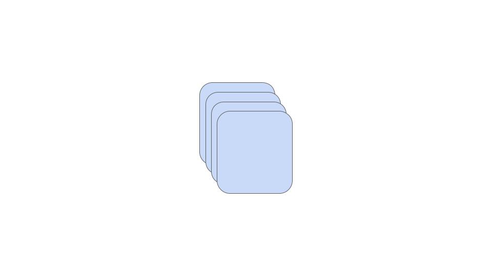
And finally, reshape to obtain hidden_large which is the same as hidden as if we had a single GPU. hidden_large contains embeddings of all images in the global batch and is shaped \(global\_batch\_size \times dim\).
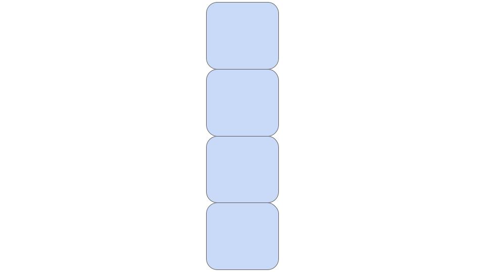
We can now compute logits_aa and logits_ab like before, the only difference is that hidden is multiplied with hidden_large
logits_ab = tf.matmul(hidden1, hidden2_large, transpose_b=True) / self.temperature
logits_aa = tf.matmul(hidden1, hidden1_large, transpose_b=True) / self.temperature
The shape of logits_ab and logits_aa is \(local\_batch\_size \times global\_batch\_size\). This way the loss is computed only on the values in each GPU local portion of the global batch, but each local positive pair is still compared against all other values in the global batch.