Movie Recommender from Pytorch to Elasticsearch

In this post I’ll train and serve a movie recommender from scratch!
I’ll use the movielens 1M dataset to train a Factorization Machine model implemented with pytorch. After learning the vector representation of movies and user metadata I’ll use elasticsearch, a production grade search engine, to serve the model and recommend movies to new users.
The full code is here: github, colab

(A short) Introduction to Factorization Machines

Factorization Machines (FM) is a supervised machine learning model that extends traditional matrix factorization by also learning interactions between different feature values of the model. An advantage of FM is that it solves the cold start problem, we can make predictions based on user metadata (age, gender etc.) even if it is a user the system has never seen before.

The input to the model is a list of events that looks like this:

FM feature matrix

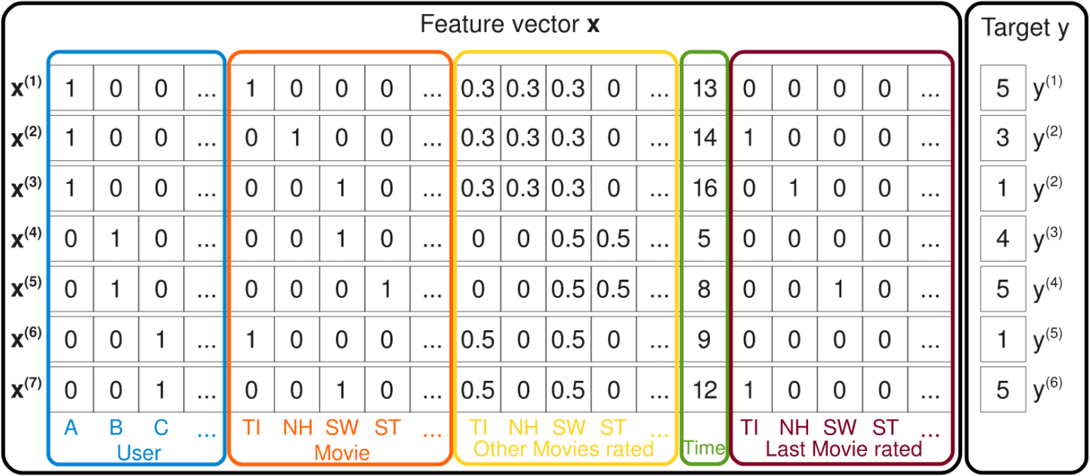
Each row is an event, for example $x^{(1)}$ is the event that user A rated movie TI at time 13 with the value $y^{(1)}=5$. Each feature value is represented by a column, for example for users we have A, B, C etc. feature values. The width of the row is the number feature values.
In this case there is some more metadata like “Last Movie rated”, but in our movielens dataset we will add user age, gender and occupation instead.

The model equation for a factorization machine of degree d=2 is defined as:

$$ \hat y(x) := w_0 + \sum_{i = 1}^n w_ix_i + \sum_{i = 1}^n\sum_{j = i + 1}^{n}\langle v_i, v_j\rangle x_ix_j $$

Each feature value (column in the input matrix) will be assigned an embeddings vector $v_i$ of size $k$ and a bias factor $w_i$ that will be learned during the training process. $\langle v_i,v_j\rangle$ models the interaction between the $i$-th and $j$-th feature values. Hopefully the embeddings will capture some interesting semantics and similar movies/users will have similar embeddings.

Pytorch FM Model

Without further ado, lets see the pytorch implementation of the formula above:

class FMModel(nn.Module):
  def __init__(self, n, k):
    super().__init__()

    self.w0 = nn.Parameter(torch.zeros(1))
    self.bias = nn.Embedding(n, 1)
    self.embeddings = nn.Embedding(n, k)

    # See https://arxiv.org/abs/1711.09160
    with torch.no_grad(): trunc_normal_(self.embeddings.weight, std=0.01)
    with torch.no_grad(): trunc_normal_(self.bias.weight, std=0.01)

  def forward(self, X):
    emb = self.embeddings(X)
    # calculate the interactions in complexity of O(nk) see lemma 3.1 from paper
    pow_of_sum = emb.sum(dim=1).pow(2)
    sum_of_pow = emb.pow(2).sum(dim=1)
    pairwise = (pow_of_sum-sum_of_pow).sum(1)*0.5
    bias = self.bias(X).squeeze().sum(1)
    return torch.sigmoid(self.w0 + bias + pairwise)*5.5

There are a few things to point out here:

I’m implementing lemma 3.1 from the paper that proves that the pairwise interactions can be done in $O(kn)$ and not $O(kn^2)$ like this:

$$ \sum_{i = 1}^n\sum_{j = i + 1}^{n}\langle v_i, v_j\rangle x_ix_j = \sum_{f=1}^k((\sum_{i=1}^{n}v_{i,f}x_i)^2-(\sum_{i=1}^{n}v_{i,f}^2x_i^2)) $$

I’m using an Embeddings layer, so the input will be a tensor of offsets and not a sparse tensor (like in the image). So $x_i$ from before can be $[0,1,0,0,1,1,0]$ but the input to the model will be $[1,4,5]$
I wrap the result with a sigmoid function to limit $\hat y(x)$ to be between 0 and 5.5. This helps the model to learn much faster.
The embeddings are initialized with a truncated normal function - This is something I’ve learned from the fastai library and improves learning speed a lot.

Prepare and Fit Data

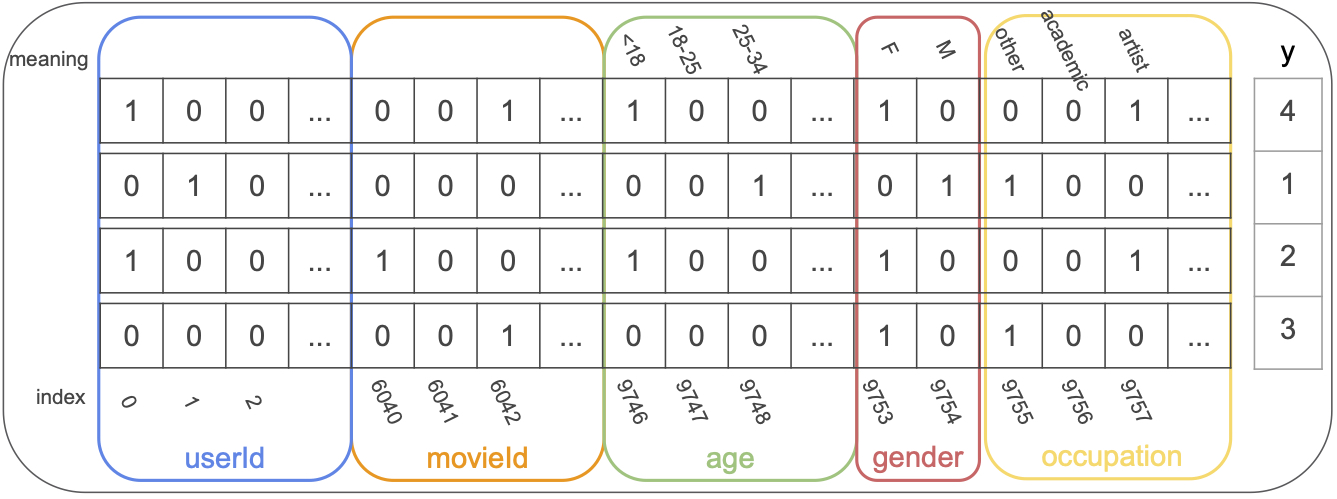
First download the 1M movielens dataset from here. After reading and chewing the data I’m left with an event input matrix like before (see code for more details):

	movieId	age	gender	occupation	rating
0	7216	9746	9753	9765	5
1	6695	9746	9753	9765	3
2	6942	9746	9753	9765	3
3	9379	9746	9753	9765	4

The numbers in the matrix represent the feature value index. I could transform each row to a sparse vector like in the paper but im using pytorch Embeddings layer that expects a list of indices. A hot encoded version of movielens input data would look like this:

movielens_input

Next step is to split the data to train and validation and create pytorch dataloader:

data_x = torch.tensor(ratings[feature_columns].values)
data_y = torch.tensor(ratings['rating'].values).float()
dataset = data.TensorDataset(data_x, data_y)
bs=1024
train_n = int(len(dataset)*0.9)
valid_n = len(dataset) - train_n
splits = [train_n,valid_n]
assert sum(splits) == len(dataset)
trainset,devset = torch.utils.data.random_split(dataset,splits)
train_dataloader = data.DataLoader(trainset,batch_size=bs,shuffle=True)
dev_dataloader = data.DataLoader(devset,batch_size=bs,shuffle=True)

Standard fit/test single epoch loops:

def fit(iterator, model, optimizer, criterion):
    train_loss = 0
    model.train()
    for x,y in iterator:
        optimizer.zero_grad()
        y_hat = model(x.to(device))
        loss = criterion(y_hat, y.to(device))
        train_loss += loss.item()*x.shape[0]
        loss.backward()
        optimizer.step()
    return train_loss / len(iterator.dataset)

def test(iterator, model, criterion):
    train_loss = 0
    model.eval()
    for x,y in iterator:                    
        with torch.no_grad():
            y_hat = model(x.to(device))
        loss = criterion(y_hat, y.to(device))
        train_loss += loss.item()*x.shape[0]
    return train_loss / len(iterator.dataset)

Create the model with $k=120$ (recall $k$ is the length of each feature value embedding), and train:

model = FMModel(data_x.max()+1, 120).to(device)
wd=1e-5
lr=0.001
epochs=10
optimizer = optim.Adam(model.parameters(), lr=lr, weight_decay=wd)
scheduler = optim.lr_scheduler.MultiStepLR(optimizer, milestones=[7], gamma=0.1)
criterion = nn.MSELoss().to(device)
for epoch in range(epochs):
  start_time = time.time()
  train_loss = fit(train_dataloader, model, optimizer, criterion)
  valid_loss = test(dev_dataloader, model, criterion)
  scheduler.step()
  secs = int(time.time() - start_time)
  print(f'epoch {epoch}. time: {secs}[s]')
  print(f'\ttrain rmse: {(math.sqrt(train_loss)):.4f}')
  print(f'\tvalidation rmse: {(math.sqrt(valid_loss)):.4f}')

After 10 epochs the rmse is 0.8532, from what I’ve seen on various leaderboards this is fine for a vanilla FM model.

Understand Embeddings

After the model finished training, each feature value has its own embedding and hopefully the model managed to capture some semantics just like word2vec does for words. I expect similar feature values, for example similar movies or users with similar taste, to be close to one another when measuring distance with cosine similarity.

To examine embeddings similarity, Ill visualize embeddings of movies in these different genres: Children's, Horror and Documentary on a 2D plot using t-SNE for dimensionality reduction:

movies_subset = movies[movies['genres'].str.contains('Children\'s|Horror|Documentary')].copy()
X = np.stack(movies_subset['embedding'].values)
ldr = TSNE(n_components=2, random_state=0)
Y = ldr.fit_transform(X)
movies_subset['x'] = Y[:, 0]
movies_subset['y'] = Y[:, 1]
ax = sns.scatterplot(x="x", y="y", hue='genres',data=movies_subset)

movie embeddings

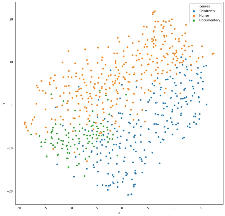
Cool! The model managed to separate genres without me telling it the real genre!
Another way to look at this is to pick a movie, print the 10 most closest movies to it and validate the closest movies are similar to the one we picked. Ill pick Toy Story and check:

toy_story_index=torch.tensor(6040,device=device)
toy_story_embeddings = model.embeddings(toy_story_index)
cosine_similarities = torch.tensor([F.cosine_similarity(toy_story_embeddings,i,dim=0) 
                                    for i in movie_embeddings])
movies.iloc[cosine_similarities.argsort(descending=True).detach().numpy()]['title'].values[:10]

['Toy Story (1995)',
 'Toy Story 2 (1999)',
 "Bug's Life, A (1998)",
 'Beauty and the Beast (1991)',
 'Aladdin (1992)',
 'Little Mermaid, The (1989)',
 'Babe (1995)',
 'Lion King, The (1994)',
 'Tarzan (1999)',
 'Back to the Future (1985)']

Nice! The model placed kids animations close to each other.

Make Movie Recommendations

We can now make movie recommendations to users we have seen in the train data and users we have not seen but know their metadata (like age, gender or occupation). All we have to do is calculate the FM equations once for each movie and see which movies get the highest predicted rating.
For example, if we have a new (never seen in train so no userId embedding) male user (male_index=9754) and his age is between 18 and 25 (age18_25_index=9747) we will calculate $\hat y(x)$ for each movie:

$$ \hat y(9754,9747,movie_i):= w_0 + w_{9747}+ w_{9754} + w_{movie_i}+ \sum_{i = \{9747,9754,movie_i\}}\sum_j \langle v_i, v_j\rangle x_ix_j $$

And choose the $movie_i$’s with the highest ratings. But the nice thing here is that for recommendation I don’t need the rating itself, it’s enough to rank movies without calculating the full equation. I can do this by ignoring all the terms in $\hat y(x)$ that are the same for all movies, and then I’m left with:

$$ score(movie_i):= w_{movie_i} +\langle v_{movie_i},v_{9754}\rangle + \langle v_{movie_i},v_{9747}\rangle $$

which is the same as

$$ score(movie_i):= w_{movie_i} + \langle (v_{9754}+v_{9747}),v_{movie_i}\rangle $$

To summarize, when a user with metadata x,y,z needs a recommendation, I will sum the metadata embeddings $v_{metadata}=v_x+v_y+v_z$ and rank all the movies by calculating:

$$ rank(movie_i):=w_{movie_i}+\langle v_{metadata},movie_i\rangle $$

Lets recommend top 10 movies to a male aged 18 to 25 new user with these steps:

Get “man” embeddings $v_{9754}$
Get “age 18 to 25” embeddings $v_{9747}$
Calculate $v_{metadata}=v_{9754} + v_{9747}$
Calculate rank for each movie and return top 10

And for the code:

man_embedding = model.embeddings(torch.tensor(9754,device=device))
age18_25_embedding = model.embeddings(torch.tensor(9747,device=device))
metadata_embedding = man_embedding+age18_25_embedding
rankings = movie_biases.squeeze()+(metadata_embedding*movie_embeddings).sum(1)
movies.iloc[rankings.argsort(descending=True)]['title'].values[:10]

['Shawshank Redemption, The (1994)',
 'Usual Suspects, The (1995)',
 'American Beauty (1999)',
 'Godfather, The (1972)',
 'Life Is Beautiful (La Vita è bella) (1997)',
 'Braveheart (1995)',
 'Sanjuro (1962)',
 'Monty Python and the Holy Grail (1974)',
 'Star Wars: Episode IV - A New Hope (1977)',
 'Star Wars: Episode V - The Empire Strikes Back (1980)']

And now lets recommend top 10 movies to a female between 50 and 56 new user:

woman_embedding = model.embeddings(torch.tensor(9753,device=device))
age50_56_embedding = model.embeddings(torch.tensor(9751,device=device))
metadata_embedding = woman_embedding+age50_56_embedding
rankings = movie_biases.squeeze()+(metadata_embedding*movie_embeddings).sum(1)
movies.iloc[rankings.argsort(descending=True)]['title'].values[:10]

['To Kill a Mockingbird (1962)',
 'Wrong Trousers, The (1993)',
 'African Queen, The (1951)',
 'Close Shave, A (1995)',
 "Schindler's List (1993)",
 'Man for All Seasons, A (1966)',
 'Some Like It Hot (1959)',
 'General, The (1927)',
 'Sound of Music, The (1965)',
 'Wizard of Oz, The (1939)']

Seems about right ¯\(ツ)/¯

Serve Recommender System with Elasticsearch

The last step in building my recommender is to move from my jupyter code to a real time serving system. I’ll use elasticsearch, an open source distributed search engine based on lucene. Lately elasticsearch introduced a new document field type called “dense_vector”, which I will use to store my feature value embeddings, and for ranking via the built in vector operations. Each feature value will be represented as a document that stores embedding $v_i$ and bias $w_i$.

After indexing all the feature value documents (see details below) this is how the recommendation flow will go:

User enters my system (netflix website for example)
Query elasticsearch for user metadata vectors and add them to create $v_{metadata}$
Query elasticsearch again, this time sending $v_{metadata}$ and ranking movies by $rank(movie_i)$
Display the results

First thing is to get elasticsearch running, creating an index and indexing all embeddings. Lets quickstart by downloading and running elasticsearch on a single node with default configurations:

curl -L -O https://artifacts.elastic.co/downloads/elasticsearch/elasticsearch-7.6.0-darwin-x86_64.tar.gz
tar -xvf elasticsearch-7.6.0-darwin-x86_64.tar.gz
cd elasticsearch-7.6.0/bin
./elasticsearch

I will now create a new index in my cluster, each document will have 4 fields, “embeddings” of type “dense_vector” this type will allow us to perform the dot product operation, “bias” is $w_i$, “feature_type” is the type of feature this doc represents (user, movie, user_metadata) and will be used for filtering, title is the name of the movie.

curl -X PUT "localhost:9200/recsys?pretty" -H 'Content-Type: application/json' -d'
{
  "mappings": {
    "properties": {
      "feature_type":{
        "type":"keyword"
      },
      "embedding": {
        "type": "dense_vector",
        "dims": 120
      },
      "bias": {
        "type":"double"
      },
      "title" : {
        "type" : "keyword"
      }
    }
  }
}
'

Back to my python notebook, I’ll now create a document from each movie and index it:

def generate_movie_docs():
    for i, movie in movies.iterrows():
        yield {
            '_index': 'recsys',
            '_id': f'movie_{movie["movieId"]}',
            '_source': {'embedding':movie['embedding'],
                    'bias':movie['bias'],
                    'feature_type':'movie',
                    'title':movie['title']
                   }
        }
es = Elasticsearch()
helpers.bulk(es,generate_movie_docs())

Ill do the same for user, age, gender and occupation vectors. The only difference between them is ‘feature_type’ which I use later for filtering results.
Ill still need to store somewhere the mapping between feature value to index (for example female index is 9753), these indices were chosen when I created the datasets. I can store them anywhere and load them to memory when the system starts.

Now everything is set, we can start making predictions according to the flow:

The same new user from before - male between 18-25 enters my website!
Query elasticsearch for user metadata vectors and sum them to create $v_{metadata}$

metadata = es.mget({"docs":[
    {
        "_index" : "recsys",
        "_id" : "age_9747"},
    {
        "_index" : "recsys",
        "_id" : "gender_9754"}]})
embeddings = [doc['_source']['embedding'] for doc in metadata['docs']]
v_metadata = [sum(pair) for pair in zip(*embeddings)]

Query elasticsearch again, this time sending $v_{metadata}$ and ranking movies by $rank(movie_i)$

search_body = {
    "query": {
    "script_score": {
      "query" : {
          "bool" : {
          "filter" : {
            "term" : {
              "feature_type" : "movie" 
            }
          }
        }
      },
      "script": {
        "source": "dotProduct(params.query_vector, \u0027embedding\u0027) + doc[\u0027bias\u0027].value", 
        "params": {
          "query_vector": v_metadata
        }
      }
    }
  }
}
[hit['_source']['title'] 
 for hit in es.search(search_body,index='recsys',_source_includes='title')['hits']['hits']]

The filter part is only for calculating movie documents.
The “source” script is the ranking method on each movie document with the v_metadata from stage 2.

And the results…

['Shawshank Redemption, The (1994)',
 'Usual Suspects, The (1995)',
 'American Beauty (1999)',
 'Godfather, The (1972)',
 'Life Is Beautiful (La Vita è bella) (1997)',
 'Braveheart (1995)',
 'Sanjuro (1962)',
 'Monty Python and the Holy Grail (1974)',
 'Star Wars: Episode IV - A New Hope (1977)',
 'Star Wars: Episode V - The Empire Strikes Back (1980)']

Awesome! we are out from a jupyter playground to a real world, production quality serving system!