Interpretable ECG Classification With 1D Vision Transformer

In this post, I will use a vision transformer to classify ECG signals and use the attention scores to interpret what part of the signal the model is focusing on. All the code to reproduce the results is in my github.

Electrocardiogram (ECG)

An ECG is a noninvasive test that records the heart’s electrical activity. This activity is the coordinated electrical impulses generated and transmitted throughout the heart’s muscle tissue, causing it to contract and pump blood. The test is performed by attaching electrodes to the skin of the chest, arms, and legs. These electrodes measure the voltage amplitude and direction of the heart activity over time.

The following animation presents the heart’s electrical activity and how an ECG records it. The red dots/lines are an electrical pulse initiating at the right atrium, causing it to contract and pump deoxygenated blood to the right ventricle. At the same time, the left atrium also contracts and pumps oxygen-rich blood to the left ventricle. The electrical pulse then reaches the atrioventricular (AV) node between the atria and ventricles and is delayed before it is sent down into the ventricular muscle. This triggers the ventricles to contract and pump blood out to the body.
The blue recording at the bottom is the voltage recorded between two electrodes during the cardiac cycle.

This is the recording of the voltage between only two electrodes, but to get a more detailed view of the heart’s activity, we attach more electrodes and measure the voltage from 12 different positions. In my mind, I imagen 12 cameras recording the heart from 12 3D locations.

The following image illustrates the locations from which the 12 leads are recorded. The lead’s names are I, II, III, aVR, aVL, v1, v2, v3, v4, v5, and v6.

The output of the ECG is the 12 leads recordings of voltage over time and looks like this (click to enlarge): 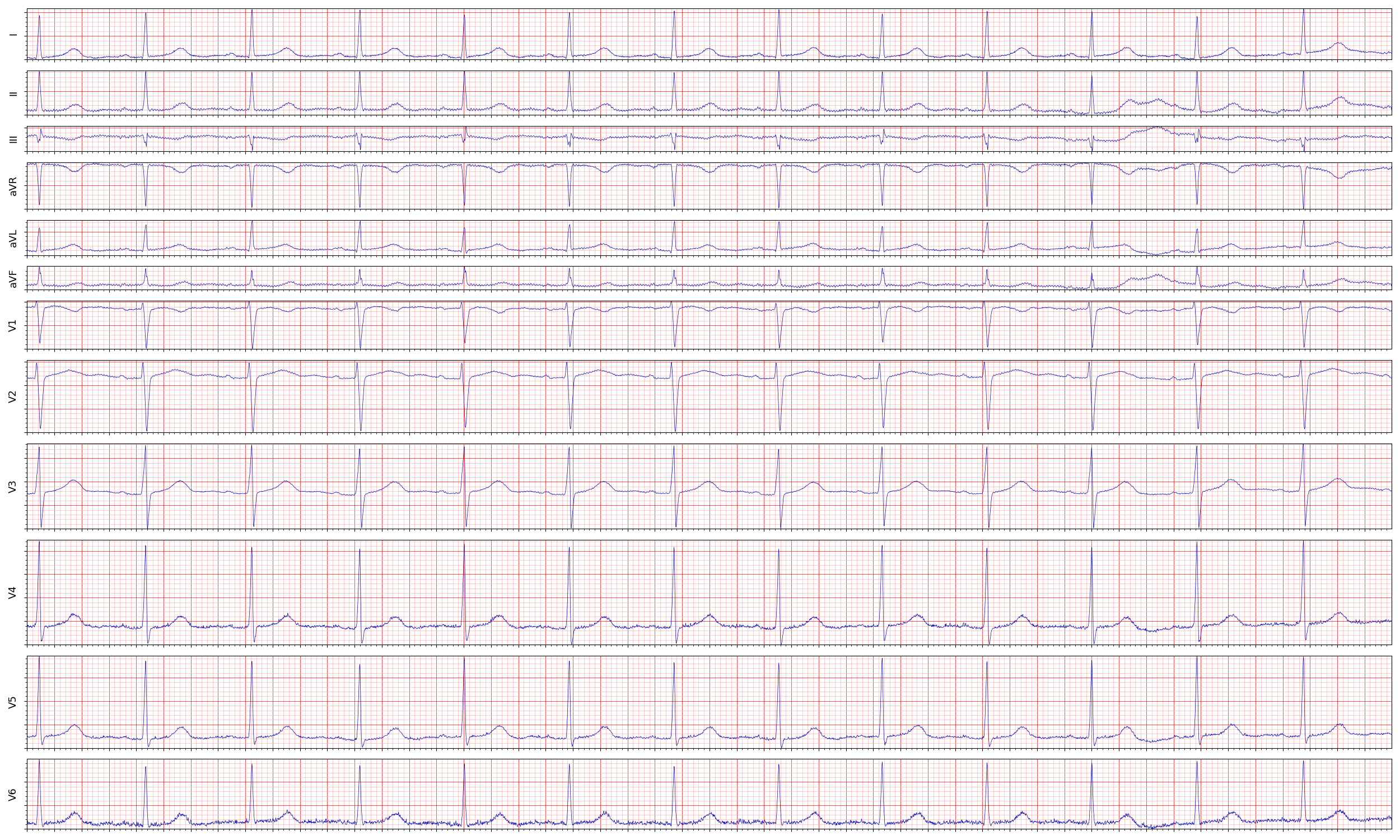As you can see, every lead records a different view of the heart’s electrical activity. Also, you can see from the previous image that leads “aVR” and “I” are recording the activity from nearly opposite positions. Similarly, If you look at the recording of “aVR” and “I” you see that the signals are opposite.

Hearbeat Complex

The cardiac cycle is the sequence of events that occur during one complete heartbeat. The different components of the cardiac cycle include:

• The P-wave.
• The QRS complex.
• The T-wave.
• The PR Interval.
• The ST segment.
• The QT interval.

The following image displays each component:

Left Ventricular Hypertrophy

Physicians use the ECG to diagnose various diseases, and during this post, I will focus on one in particular: “Left Ventricular Hypertrophy” (LVH). LVH is a condition where (as the name suggests :) ) there is hypertrophy of the left ventricle heart muscle. Hypertrophy means a thickening of muscle tissue, and Left Ventricular Hypertrophy means a thickening of the muscle tissue of the left ventricle. The thickened heart tissue causes the ventricle lumen to be smaller and the left ventricular heart muscle to be less elastic, making it harder to pump blood to the rest of the body.

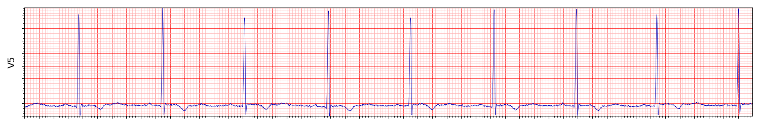
The manifestation of LVH in ECG exams is high voltage because the increased muscle mass of the left ventricle generates a larger electrical current, which results in a taller QRS complex. Another indication is inverted T waves. Here is an example of lead V5 from a patient with LVH (More on the dataset later). The R peaks are high, and the T waves are inverted:

After this short introduction to ECG, it’s time to train our model

Data

I’m going to use this dataset which contains 45152 12 lead ECGs. Each ECG comes with a list of labels described here. The file contains descriptions of many conditions, but I am only interested in two: LVH and TWO (T-Wave Opposite).
The first step is to parse the files in the dataset and create a dataframe representing the training data. This function parses all the files, looks for the LVH and TWO, labels, and builds the dataframe. To simplify, I take all the LVH/TWO ECGs and sample only 20000 negative ECGs. Finally, I split the data to train/test using a hash function on the filename. The resulting dataframe contains the file path, y label, which is the hot encoding of LVH and TWO, and test, which indicates validation data:

file	y	test
<root_path>/WFDBRecords/34/342/JS33623	[0. 0.]	True
<root_path>/WFDBRecords/42/425/JS41970	[0. 0.]	False
<root_path>/WFDBRecords/02/024/JS01566	[0. 0.]	False
<root_path>/WFDBRecords/42/424/JS41856	[0. 0.]	False
<root_path>/WFDBRecords/22/220/JS21462	[1. 0.]	False
<root_path>/WFDBRecords/32/329/JS32343	[0. 0.]	False

Note: It’s better to split train/test by hash and not some random function to get the same split every time. Setting the random seed is not enough because if I add even one sample to the train, the whole train/test split will be different.

I use the wfdb library to parse the files into an np.array representing the ECG. The np.array shape is (5000,12) - 5000 samples of 12 leads. In this dataset the sampling rate is 500, meaning the length of each ECG is 10 seconds.

record = wfdb.rdrecord(df["file"].values[0])
print(record.p_signal.shape)
print(record.fs)

> (5000, 12)
> 500

Now I can create the TensorFlow train/val datasets. Nothing special here; shuffle, open files, batch, and prefetch.

def read_record(path):
    record = wfdb.rdrecord(path.decode("utf-8"))
    return record.p_signal.astype(np.float32)

def ds_base(df, shuffle, bs):
    ds = tf.data.Dataset.from_tensor_slices((df["file"], list(df["y"])))
    if shuffle:
        ds = ds.shuffle(len(df))
    ds = ds.map(
        lambda x, y: (tf.numpy_function(read_record, inp=[x], Tout=tf.float32), y),
        num_parallel_calls=tf.data.AUTOTUNE,
        deterministic=False,
    )
    ds = ds.map(lambda x, y: (tf.where(tf.math.is_nan(x), tf.zeros_like(x), x), y)) 
    ds = ds.map(lambda x, y: (tf.ensure_shape(x, [5000, 12]), y))
    ds = ds.batch(bs)
    ds = ds.prefetch(tf.data.AUTOTUNE)
    return ds

def gen_datasets(df, bs):
    train_ds = ds_base(df[~df["test"]], True, bs)
    val_ds = ds_base(df[df["test"]], False, bs)
    return train_ds, val_ds

Model - 1D Vision Transformer

The model is a vision transformer with a minor change; the patches are not 2D 16x16, but 1D sized 20. Twenty samples represent 0.04[sec], precisely one small square on the ECG image. The small squares are the standard granularity used for diagnosis, so it makes sense for that to be the patch size. The Conv filter size is 20, but the number of channels in the signal is 12, so each patch is sized 20 across all leads (channels).

Let’s start with the embeddings layer. The input is an (5000,12) ECG array, and the layer will create embeddings for 5000/patch_size+1 patches (including the cls_token). Then, add positional embeddings and return a tensor shaped (bs,5000/patch_size+1,hidden_size).

class ViTEmbeddings(tf.keras.layers.Layer):
    def __init__(self, patch_size, hidden_size, dropout=0.0, **kwargs):
        super().__init__(**kwargs)

        self.patch_size = patch_size
        self.hidden_size = hidden_size

        self.patch_embeddings = tf.keras.layers.Conv1D(filters=hidden_size, kernel_size=patch_size, strides=patch_size)
        self.dropout = tf.keras.layers.Dropout(rate=dropout)

    def build(self, input_shape):
        self.cls_token = self.add_weight(shape=(1, 1, self.hidden_size), trainable=True, name="cls_token")

        num_patches = input_shape[1] // self.patch_size
        self.position_embeddings = self.add_weight(
            shape=(1, num_patches + 1, self.hidden_size), trainable=True, name="position_embeddings"
        )

    def call(self, inputs: tf.Tensor, training: bool = False) -> tf.Tensor:
        inputs_shape = tf.shape(inputs)  # N,H,W,C
        embeddings = self.patch_embeddings(inputs, training=training)

        # add the [CLS] token to the embedded patch tokens
        cls_tokens = tf.repeat(self.cls_token, repeats=inputs_shape[0], axis=0)
        embeddings = tf.concat((cls_tokens, embeddings), axis=1)

        # add positional encoding to each token
        embeddings = embeddings + self.position_embeddings
        embeddings = self.dropout(embeddings, training=training)

        return embeddings

Next is the MLP; nothing special here. It is the same as in the vit paper.

class MLP(tf.keras.layers.Layer):
    def __init__(self, mlp_dim, out_dim=None, activation="gelu", dropout=0.0, **kwargs):
        super().__init__(**kwargs)
        self.mlp_dim = mlp_dim
        self.out_dim = out_dim
        self.activation = activation
        self.dropout_rate = dropout

    def build(self, input_shape):
        self.dense1 = tf.keras.layers.Dense(self.mlp_dim)
        self.activation1 = tf.keras.layers.Activation(self.activation)
        self.dropout = tf.keras.layers.Dropout(self.dropout_rate)
        self.dense2 = tf.keras.layers.Dense(input_shape[-1] if self.out_dim is None else self.out_dim)

    def call(self, inputs: tf.Tensor, training: bool = False):
        x = self.dense1(inputs)
        x = self.activation1(x)
        x = self.dropout(x, training=training)
        x = self.dense2(x)
        x = self.dropout(x, training=training)
        return x

The main encoder block. Normalization layers, attention layer, and MLP are all connected with skip connections with a stochastic depth layer. Each block has an additional function, get_attention_scores, that isn’t called during training. get_attention_scores is used only to get the attention weights from the attention layer, and I will use it later for interpretability.

class Block(tf.keras.layers.Layer):
    def __init__(
        self,
        num_heads,
        attention_dim,
        attention_bias,
        mlp_dim,
        attention_dropout=0.0,
        sd_survival_probability=1.0,
        activation="gelu",
        dropout=0.0,
        **kwargs,
    ):
        super().__init__(**kwargs)
        self.norm_before = tf.keras.layers.LayerNormalization()
        self.attn = tf.keras.layers.MultiHeadAttention(
            num_heads,
            attention_dim // num_heads,
            use_bias=attention_bias,
            dropout=attention_dropout,
        )
        self.stochastic_depth = tfa.layers.StochasticDepth(sd_survival_probability)
        self.norm_after = tf.keras.layers.LayerNormalization()
        self.mlp = MLP(mlp_dim=mlp_dim, activation=activation, dropout=dropout)

    def build(self, input_shape):
        super().build(input_shape)
        # TODO YONIGO: tf doc says to do this  ¯\_(ツ)_/¯
        self.attn._build_from_signature(input_shape, input_shape)

    def call(self, inputs, training=False):
        x = self.norm_before(inputs, training=training)
        x = self.attn(x, x, training=training)
        x = self.stochastic_depth([inputs, x], training=training)
        x2 = self.norm_after(x, training=training)
        x2 = self.mlp(x2, training=training)
        return self.stochastic_depth([x, x2], training=training)

    def get_attention_scores(self, inputs):
        x = self.norm_before(inputs, training=False)
        _, weights = self.attn(x, x, training=False, return_attention_scores=True)
        return weights

Finally, I tie everything together in the VisionTransformer model:

class VisionTransformer(tf.keras.Model):
    def __init__(
        self,
        patch_size,
        hidden_size,
        depth,
        num_heads,
        mlp_dim,
        num_classes,
        dropout=0.0,
        sd_survival_probability=1.0,
        attention_bias=False,
        attention_dropout=0.0,
        *args,
        **kwargs,
    ):
        super().__init__(*args, **kwargs)

        self.embeddings = ViTEmbeddings(patch_size, hidden_size, dropout)
        sd = tf.linspace(1.0, sd_survival_probability, depth)
        self.blocks = [
            Block(
                num_heads,
                attention_dim=hidden_size,
                attention_bias=attention_bias,
                attention_dropout=attention_dropout,
                mlp_dim=mlp_dim,
                sd_survival_probability=(sd[i].numpy().item()),
                dropout=dropout,
            )
            for i in range(depth)
        ]

        self.norm = tf.keras.layers.LayerNormalization()

        self.head = tf.keras.layers.Dense(num_classes)

    def call(self, inputs: tf.Tensor, training: bool = False) -> tf.Tensor:
        x = self.embeddings(inputs, training=training)
        for block in self.blocks:
            x = block(x, training=training)
        x = self.norm(x)
        x = x[:, 0]  # take only cls_token
        return self.head(x)

    def get_last_selfattention(self, inputs: tf.Tensor):
        x = self.embeddings(inputs, training=False)
        for block in self.blocks[:-1]:
            x = block(x, training=False)
        return self.blocks[-1].get_attention_scores(x)

Train

Create ViT and train!

vit = VisionTransformer(
    patch_size=20,
    hidden_size=768,
    depth=6,
    num_heads=6,
    mlp_dim=256,
    num_classes=len(df["y"].values[0]),
    sd_survival_probability=0.9,
)

optimizer = tf.keras.optimizers.Adam(0.0001)
loss = tf.keras.losses.BinaryCrossentropy(from_logits=True)
metrics = [tf.keras.metrics.AUC(from_logits=True, name="roc_auc")]
vit.compile(optimizer=optimizer, loss=loss, metrics=metrics)

cbs = [tf.keras.callbacks.ModelCheckpoint("vit_best/", monitor="val_roc_auc", save_best_only=True, save_weights_only=True)]

vit.fit(train_ds, validation_data=val_ds, epochs=10, callbacks=cbs)

The average AUC of the roc curve on the validation set is 0.95. This performance metric means nothing in the context of this blog post except that it is much better than random, and the model probably learned something. Is this result good or bad depends on other factors such as product definition, human-level performance on the task, and other benchmarks on the same or related tasks. I can improve performance by using more data, labels, augmentations, and signal preprocessing, such as cleaning high-frequency noise and low-frequency trends. But, the goal of this experiment is not to achieve SOTA using ViT but to see if I can use ViT for interpretability.

Interpetability

Finally, the main course of this post! Did the model learn something meaningful? is it focusing on the same parts of the ECG as physicians do to detect LVH??? Remember, physicians look for high QRS complexes and inverted T-waves. I added to the ViT implementation a function get_last_selfattention. This function does a complete forward pass on all the layers except for the last block, on which it just calls get_attention_scores to return the attention scores from the MultiHeadAttention layer.

record = wfdb.rdrecord(file_path)
attn = vit.get_last_selfattention(tf.expand_dims(record.p_signal, 0))
print(attn.shape)
> (1, 6, 251, 251)

The attn scores is shaped (batch_size, num_heads, num_patches, num_patches). The fully connected classification head at the end of the model is feeded only by the cls_token embedding, so I’m interested in the attention scores of all the other 250 patches when the last attention layer calculated the cls_token output. The cls_token embedding is the first from the 251 (that’s just how I did it in the VitEmbeddings layer), so for each of the 6 heads, I take row 0 and skip column 0 because I’m not interested in the score of the cls_token on itself:

attn = attn[0, :, 0, 1:]
print(attn.shape)
> (6, 250)

Now the attn contains the score of all 250 patches for each head. To display these scores on an ECG, I need to resize the 250 back to 5000. Each patch represents 20 samples from the ECG, so I need to repeat each score 20 times.

attn = tf.transpose(attn, (1, 0))
attn = tf.expand_dims(tf.expand_dims(attn, 0), 0)
attn = tf.image.resize(attn, (1, 5000))[0,0]
print(attn.shape)
> (5000, 6)

That’s it! I can now plot an ECG lead and display the scores on top of it. In pyplot, I use cmap=Reds so that it colors high scores in darker red, and here are plots of scores from different attention heads:

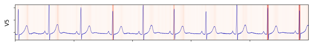
The first head learned to pay attention to the T-Wave, and the second to the QRS complex! The rest of the heads were a mix of QRS and T, so I didn’t include them. It’s also interesting to see the second head paying the most attention to the two last heartbeats. There is redundancy in these signals as the heartbeats don’t vary much, so maybe the model learns to focus only on some of them.

---

Thats it! Not only can I use the model for ECG classification, but I can also explain what parts of the ECG the model pays attention to.