Some time ago, with the explosion of DALLE2 and stable diffusion, I also wanted to understand how these models tick, so I opened the Denoising Diffusion Probabilistic Models (DDPM) paper. At the very beginning, I encountered this line:

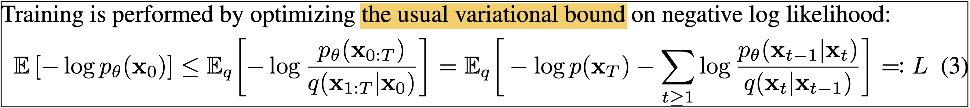
“the usual variational bound”…

Ok, this “variational bound” is “usual” for these people. Clearly, I need to catch up with some of these concepts. In this post, Ill start from the very beginning - Variational Auto Encoders (VAE). I’ll derive ELBO and construct the VAE model and loss. Then, I will jump five years back to the DDPM paper, show why the objective is “usual”, and discuss how it differs from the classic VAE.

VAE - Problem Scenario

This is the VAE graphical model

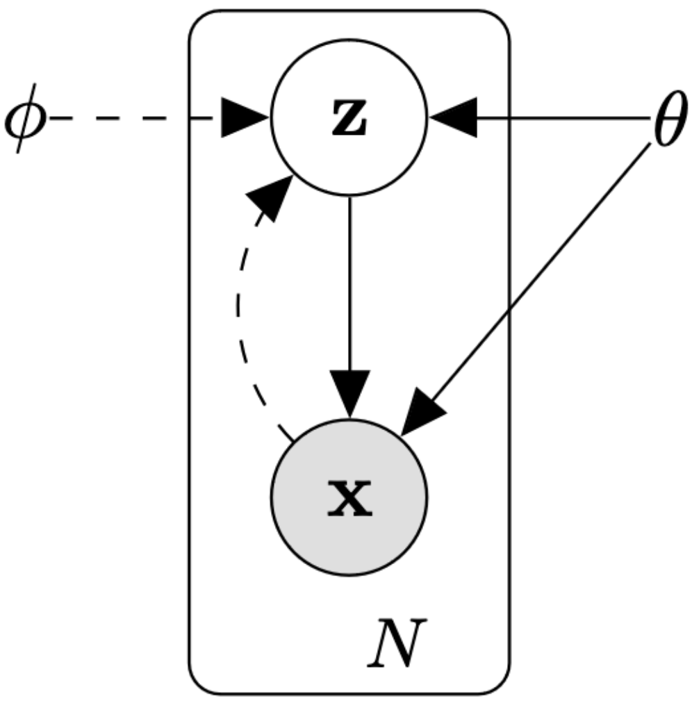
$X=\{x^{(i)}\}_{i=0}^N$ is our observed dataset, For example, N i.i.d images of cats. These images came from an unknown distribution $p_\theta(\mathbf{x})$, which describes all the images of cats in the world. $\mathbf z$ is a latent variable that follows the distribution $p_\theta(\mathbf{z})$. We assume that every cat image was generated with these steps:

Draw $z^{(i)}$ from $p_\theta(\mathbf{z})$
Generate $x^{(i)}$ from the conditional distribution $p_\theta(\mathbf{x}\vert \mathbf{z})$

I want to visualize this to give some better intuition:

This process means that every cat image $x^i$ has a low dimensional representation $z^i$, and from $z^i$ we can generate the image by sampling $p_\theta(\mathbf{x}\vert \mathbf{z})$. The fact that every cat has a low-dimensional representation shouldn’t surprise us; we usually see the opposite process when we use neural nets. For example, when we train a convnet, the convnet will learn to represent an image $x^i$ in a lower dimensional space $z^i$ and then pass $z^i$ through a classification layer.

Unfortunately, we do not know what the parameters $\theta$ in $p_\theta(\mathbf{x}\vert \mathbf{z})$ and $p_\theta(\mathbf{z})$ are. If we knew, we could use them to generate infinite images of random cats using the steps from above.

To find the optimal $\theta$ to make $p_\theta(\mathbf{x}\vert \mathbf{z})$ and $p_\theta(\mathbf{z})$ represent our dataset, we need to do what we always do in machine learning, try to estimate $p_\theta(\mathbf{x})$ with maximum likelihood. In other words, We need to find the parameters $\theta$ that maximize

\[\theta^*=\underset{\theta}{\operatorname{arg max}} \prod^{i=N}_{i=0} p_\theta (x^{(i)})\]

or, more commonly

\[\theta^*=\underset{\theta}{\operatorname{arg max}} \sum^{i=N}_{i=0} \log p_\theta (x^{(i)})\]

Note: A good explanation of maximum likelihood in machine learning can be found in the “Deep Learning” book by Goodfellow chapter 5.5

Now we need to define $p_\theta(\mathbf{x})$. The probability of drawing an image $x$ in this graphical model is

\[p_\theta(\mathbf{x})= \displaystyle \int_{z}p_\theta(\mathbf{z})p_\theta(\mathbf{x}\vert \mathbf{z})dz\]

Let’s think about what this means. To calculate the probability of a specific image of a cat $p(x^{(i)})$, we must go over all of $z$ and calculate the probability of generating $x^{(i)}$ given $z$.
Of course, going over all possible values of $z$ is not something we can do, so we call $p_\theta(\mathbf{x})$ intractable, and this intractability is one of the central problems in bayesian statistics.

There are several approaches to solving this intractability, one of them is variational inference, and the intuition behind this approach is the following. For a specific image $x^{(i)}$, there is a tiny area in $z$ with a high probability of generating $x^{(i)}$. For all other $z$, the probability is close to 0. For example, think about the image of the black cat from above; there is probably a tiny region in $z$ that represents black cats with the head on the left and two open eyes. The probability of generating this black cat from the area representing white cats is ~0.

The key idea is instead of integrating all of $z$, we compute $p_\theta(x^{(i)})$ just by sampling from the tiny area in $z$, which is most likely to generate $x^{(i)}$. To find the area in $z$ most probable of generating $x^{(i)}$, we need the posterior $p_\theta(\mathbf{z}\vert \mathbf{x})$. Unfortunately, the posterior is hidden from us, but! we can estimate it with a model $q_\phi(\mathbf{z}\vert \mathbf{x})$ called the probabilistic encoder.

This is starting to get the shape of a VAE:

With this model, we will compute $p_\theta(x^{(i)})$ by first passing $x^{(i)}$ through the probabilistic encoder $q_\phi(\mathbf{z}\vert \mathbf{x})$, and the output will be a small distribution over a tiny area in $z$. Then, we sample from that distribution and compute $p_\theta(\mathbf{x}\vert \mathbf{z})$ on the samples. I’ll get into these details later.

Deriving the Objective - ELBO

Our juerney begins with the unknown posterior $p_\theta(\mathbf{z}\vert \mathbf{x})$ and our estimation of it $q_\phi(\mathbf{z}\vert \mathbf{x})$. We want our estimation to be as close to the true posterior as possible, and we can measure the distance between them using Kullback–Leibler divergence.

Note: Best intuition of KL-divergence is shown in this video

I will start by writing the KL-divergence between $q_\phi(\mathbf{z}\vert \mathbf{x})$ and $p_\theta(\mathbf{z}\vert \mathbf{x})$ and do some basic arithmentics on the equation.

$$\begin{eqnarray} D_{KL}[q_\phi(\mathbf{z}\vert \mathbf{x})||p_\theta(\mathbf{z}\vert \mathbf{x})] &=& \mathbb{E}_{z\sim q_\phi}[\log q_\phi(\mathbf{z}\vert \mathbf{x})-\log p_\theta(\mathbf{z}\vert \mathbf{x})] \qquad &;& 1 \\ D_{KL}[q_\phi(\mathbf{z}\vert \mathbf{x})||p_\theta(\mathbf{z}\vert \mathbf{x})] &=& \mathbb{E}_{z\sim q_\phi}[\log q_\phi(\mathbf{z}\vert \mathbf{x})-\log {p_\theta(\mathbf{x}\vert \mathbf{z})p_\theta(\mathbf{z})\over \log p_\theta(\mathbf{x})}] &;& 2\\ D_{KL}[q_\phi(\mathbf{z}\vert \mathbf{x})||p_\theta(\mathbf{z}\vert \mathbf{x})] &=& \mathbb{E}_{z\sim q_\phi}[\log q_\phi(\mathbf{z}\vert \mathbf{x})-\log p_\theta(\mathbf{x}\vert \mathbf{z})-\log p_\theta(\mathbf{z})-\log p_\theta(\mathbf{x})] &;& 3 \\ D_{KL}[q_\phi(\mathbf{z}\vert \mathbf{x})||p_\theta(\mathbf{z}\vert \mathbf{x})] &=& \mathbb{E}_{z\sim q_\phi}[\log q_\phi(\mathbf{z}\vert \mathbf{x})-\log p_\theta(\mathbf{x}\vert \mathbf{z})-\log p_\theta(\mathbf{z})]-\log p_\theta(\mathbf{x}) &;& 4\\ D_{KL}[q_\phi(\mathbf{z}\vert \mathbf{x})||p_\theta(\mathbf{z}\vert \mathbf{x})]-\log p_\theta(\mathbf{x})&=& -\mathbb{E}_{z\sim q_\phi}[\log p_\theta(\mathbf{x}\vert \mathbf{z})]+D_{KL}[q_\phi(\mathbf{z}\vert \mathbf{x}) \vert\vert p_\theta(\mathbf{z})] &;& 5\\ \\ \log p_\theta(\mathbf{x})-D_{KL}[q_\phi(\mathbf{z}\vert \mathbf{x})||p_\theta(\mathbf{z}\vert \mathbf{x})] &=& \mathbb{E}_{z\sim q_\phi}[\log p_\theta(\mathbf{x}\vert \mathbf{z})]-D_{KL}[\log q_\phi(\mathbf{z}\vert \mathbf{x}) \vert\vert\ p_\theta(\mathbf{z})] &;& 6\\\\ \log p_\theta(\mathbf{x})&\ge& \mathbb{E}_{z\sim q_\phi}[\log p_\theta(\mathbf{x}\vert \mathbf{z})]-D_{KL}[q_\phi(\mathbf{z}\vert \mathbf{x}) \vert\vert p_\theta(\mathbf{z})] &;& 7\\\\ \end{eqnarray}$$

Definition of KL-divergence.
Bayes rule.
Log rules.
$p_\theta(\mathbf{x})$ does not depend on $z$ so can be taken out of $\mathbb{E_z}$
Definition of KL-divergence.

Variational Lower Bound (ELBO)

(6) and (7) can be visualised like this

We want to maximize the likelihood of $\log p_\theta(\mathbf{x})$ (the evidence), which is intractable. $D_{KL}[q_\phi(\mathbf{z}\vert \mathbf{x})\vert\vert p_\theta(\mathbf{z}\vert \mathbf{x})]$ is also intractable, but, the evidence/variational lower bound (ELBO) is computable and can be maximized via gradient descent. By maximizing the lower bound we are also pushing $\log p_\theta(\mathbf{x})$ up, because $D_{KL}[q_\phi(\mathbf{z}\vert \mathbf{x})\vert\vert p_\theta(\mathbf{z}\vert \mathbf{x})]$ is always positive.
Ok, so this is the “usual variational bound” the paper referred to. I will return to that later and show how the ddpm formula is the same as (6), but first, I will finish with the original VAE.

Optimizing ELBO

Like always, instead of maximizing the ELBO term, we will minimize the -ELBO, so our loss function is

$$\mathcal{L}(\theta,\phi;\mathbf x^{(i)})= D_{KL}[q_\phi(\mathbf z\vert \mathbf x^{(i)}) \vert\vert p_\theta(\mathbf{z})]-\mathbb{E}_{z\sim q_\phi(\mathbf z\vert \mathbf x^{(i)})}[\log p_\theta(\mathbf x^{(i)}\vert \mathbf z)]$$

This is the loss of a single image $x^{(i)}$ from our dataset. Its not exactly clear how this formula becomes an explicit differentiable computation written in code, so lets break it into pieces.
First of all, the full schema of the VAE looks like:

source: wikipedia

The Probabilistic Encoder

The goal of the encoder $\log q_\phi(\mathbf z\vert \mathbf x^{(i)})$ is to estimate $\log p_\theta(\mathbf z\vert \mathbf x^{(i)})$. We are going to assume the prior $\log p_\theta(\mathbf{z})$ is centered isotropic multivariate Gaussian $\mathcal{N}(z,0,I)$ and $p_\theta(\mathbf{z}\vert \mathbf{x})$ is a multivariate Gaussian.
The approximate posterior $\log q_\phi(\mathbf z\vert \mathbf x^{(i)})$ will be a multivariate Gaussian with a diagonal covariance structure:

\[\log q_\phi(\mathbf z\vert \mathbf x^{(i)})=\mathcal{N}(\mathbf z,\mu (\mathbf x^{(i)}),\sigma ^2 (\mathbf x^{(i)})I)\]

$\mu$ and $\sigma^2$ are our two outputs from our deterministic neural net. In case $q$ and $p$ are Gaussians, $D_{KL}[q_\phi(\mathbf z\vert \mathbf x^{(i)}) \vert\vert p_\theta(\mathbf{z})]$ has an analyitical solution (appendix B in VAE paper):

$$D_{KL}[q_\phi(\mathbf z\vert \mathbf x^{(i)}) \vert\vert p_\theta(\mathbf{z})] = -{1 \over 2}\sum^{J}_{j=1}(1+\log((\sigma_j)^2)−(\mu_j )^2 − (\sigma_j )^2 )$$

So we can write the first term in the loss function as ($J$ is the dimension of $z$):

def kl_loss(mean, log_var):
    return -0.5 * tf.reduce_sum(1 + log_var - tf.square(mean) - tf.exp(log_var), axis=1)

mean, log_var = encoder(x)
loss1 = kl_loss(mean, log_var)

Instead of the encoder outputting $\sigma^2$ its better to output $\log(\sigma^2)$ for numerical reasons.

The Probabilistic Decoder

The second part of the loss $-\mathbb{E}_{\mathbf z\sim q_\phi(\mathbf z\vert \mathbf x^{(i)})}[\log p_\theta(\mathbf x^{(i)}\vert \mathbf z)]$ seems more intimidating. The are three unclear issues before implementing this in code:

How is the probabilistic decoder $p_\theta(\mathbf x^{(i)}\vert \mathbf z)$ modeled
How can we sample $\mathbf z$ from the output of the encoder $\mathbf z\sim q_\phi(\mathbf z\vert \mathbf x^{(i)})$ in a differntiable manner
How to deal with the $\mathbb{E}$ term

The VAE paper suggests two models for $\log p_\theta(x^{(i)}\vert z)$, Bernoulli in case of binary data an Gaussian in case of real-valued data. In the Gaussian case, the decoder is modeled as

\[p_\theta(\mathbf x^{(i)}\vert \mathbf z) = \mathcal{N}(\mathbf x,f(z) ,I)\]

$f$ is our deterministic neural net, and $z$ is a single sample from our output distribution of the encoder $z\sim \mathcal{N}(z,\mu (x^{(i)}),\sigma ^2 (x^{(i)})I)$. When modeling the decoder as a Gaussian, the term $\log p_\theta(x^{(i)}\vert z)$ in the loss becomes a simple MSE beteen $f(z)$ and $x$. If it is not clear why a Gaussian model dictates an MSE loss, refer to chapter 5.5.1 in the "Deep Learning" book.

Sampling $z$ from the output of the encoder $(\mu, \sigma^2)$ is not a differential operation, so the authors suggest the “reparameterization trick”. Instead of sampling streigt from $\mathcal{N}(\mu,\sigma^2I)$, we sample $\epsilon$ from $\epsilon \sim \mathcal{N}(0,I)$, and compute $z=\mu+\sigma\epsilon$. Backpropagation doesn’t flow back through the sampling operation and treats $e$ as a constant.

Instead of computing $\mathbb{E}_{z\sim q_\phi(z\vert x^{(i)})}$, the authors suggest sampling only $L$ $z$ values, so the second term in the loss becomes:

\[-{1\over L}\sum_{l=1}^L{\log p_\theta(x^{(i)}\vert z^{(i,l)})}\]

As $q_\phi(\mathbf z\vert \mathbf x^{(i)})$ becomes better, the $\mathbf z$ samples will become closer to the actual $\mathbf z^{(i)}$, which is the source of $\mathbf x^{(i)}$. Next, the authors even argue it’s enough to take $L=1$, which makes sense because in stochastic gradient descent, every $\mathbf x^{(i)}$ will pass through the model multiple times, and a different sample $\mathbf z$ is drawn each time.

To sum up, our loss for each $x^{(i)}$ is the kl_loss, and after we draw a single sample $z$, the MSE between the output of the decoder and $x^{(i)}$.

Back to the (DDPM) Future

The graphical model used in the ddpm paper is:

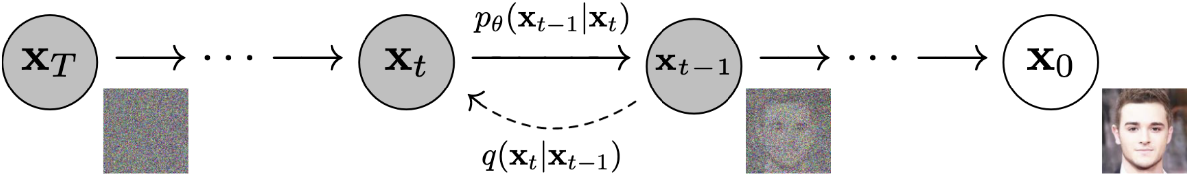
Like with VAEs, every image $x_0^{i}$ from our dataset originated from a prior distribution $p(\mathbf{x}_T)$. Instead of a single-step generation $p_\theta(\mathbf{x}\vert \mathbf{z})$ like in VAEs, DDPM generation is an iterative process defined by a Markov chain. Each step in the generation process (called revearse process in the paper) is defined by a latent variable $\mathbf{x}_t$ similar to $\mathbf{z}$ in the VAE. The transition between latent variables is defined by $p_\theta(\mathbf{x}_{t-1}\vert \mathbf{x}_t)$, which is similar to $p_\theta(\mathbf{x}\vert \mathbf{z})$ from VAEs.

The difference between diffusion models and VAEs is the approximate posterior. In VAEs, the posterior $p_\theta(\mathbf{z}\vert \mathbf{x})$ is an unknown distribution we had to approximate with a neural network. We used the probabilistic encoder to approximate the latent $\mathbf{z}$ given $\mathbf{x}$. In diffusion models, the approximate posterior $q(\mathbf{x}_{1:T}\vert \mathbf{x}_0)$, called the forward process or diffusion process, is defined by gradually adding Gaussian noise at each step $t$. So we don’t need an encoder neural net or other learnable parameters.
$q(\mathbf{x}_{1:T}\vert \mathbf{x}_0)$ is the joint probability of all latent variables $\mathbf{x}_1\colon \mathbf{x}_T$ given the original image $\mathbf{x}_0$ and is defined by

$$\begin{eqnarray} q(\mathbf{x}_{1:T}\vert \mathbf{x}_0) \colon= \prod^{T}_{t=1}p_\theta(\mathbf{x}_t\vert \mathbf{x}_{t-1}) \qquad p_\theta(\mathbf{x}_t\vert \mathbf{x}_{t-1})\colon=\mathcal{N}( \mathbf{x}_t;\sqrt{1-\beta_t} \mathbf{x}_{t-1},\beta_tI) \end{eqnarray}$$

The joint distribution of all the Markov chain latent variables together with the image $\mathbf{x}_0$ is equivalent to $p_\theta(x,z)$ in VAEs and defined by

$$\begin{eqnarray} p_\theta( \mathbf{x}_{0:T}) \colon= p( \mathbf{x}_T)\prod^{T}_{t=1}p_\theta( \mathbf{x}_{t-1}\vert \mathbf{x}_{t}) \qquad p_\theta( \mathbf{x}_{t-1}\vert \mathbf{x}_t)\colon=\mathcal{N}( \mathbf{x}_{t-1};\mu_\theta( \mathbf{x}_t,t),\Sigma_\theta( \mathbf{x}_t,t)) \end{eqnarray}$$

Now, lets look at equation (7) from above:

\[\log p_\theta(\mathbf{x})\ge \mathbb{E}_{z\sim q_\phi}[\log p_\theta(\mathbf{x}\vert \mathbf{z})] -D_{KL}[q_\phi(\mathbf{z}\vert \mathbf{x}) \vert \vert p_\theta(\mathbf{z})]\]

And do some basic arithmetics on it:

$$\begin{eqnarray} \log p_\theta(\mathbf{x})&\ge& \mathbb{E}_{z\sim q_\phi}[\log p_\theta(\mathbf{x}\vert \mathbf{z})]-\mathbb{E}_{z\sim q_\phi}[\log q_\phi(\mathbf{z}\vert \mathbf{x})]+ \mathbb{E}_{z\sim q_\phi}[\log p_\theta(\mathbf{z})] \qquad &;& {\displaystyle D_{\text{KL}}}\\ \log p_\theta(\mathbf{x})&\ge& \mathbb{E}_{z\sim q_\phi}[\log p_\theta(\mathbf{x}\vert \mathbf{z})-\log q_\phi(\mathbf{z}\vert \mathbf{x})+ \log p_\theta(\mathbf{z})] \qquad \\ \log p_\theta(\mathbf{x})&\ge& \mathbb{E}_{z\sim q_\phi}[ \log {p_\theta(\mathbf{x}\vert \mathbf{z})p_\theta(\mathbf{z}) \over q_\phi(\mathbf{z}\vert \mathbf{x})}] \qquad &;& \text{log} \\ \log p_\theta(\mathbf{x})&\ge& \mathbb{E}_{z\sim q_\phi}[ \log {p_\theta(x,z) \over q_\phi(\mathbf{z}\vert \mathbf{x})}] \qquad &;& \text{bayes} \\ \end{eqnarray}$$

The joint distribution $p_\theta(x,z)$ is equivalent to the DDPM $p_\theta( \mathbf{x}_{0:T})$, and the postirior $q_\phi(\mathbf{z}\vert \mathbf{x})$ is equivalent to the DDPM postirior $q(\mathbf{x}_{1:T}\vert \mathbf{x}_0)$. I will do these replacements and negate both sides:

\[- \log p_\theta(\mathbf{x})\le \mathbb{E}_{z\sim q_\phi} \left[ - \log {p_\theta( \mathbf{x}_{0:T}) \over q(\mathbf{x}_{1:T}\vert \mathbf{x}_0)}\right ]\]

… The usual variational bound …

Final Thoughts

After fully understanding variational auto encoders, I can finally understand the first page of the DDPM paper. Both VAEs and DDPMs are graphical models with intractable computations, and for both, we optimize the variational lower bound to maximize $\log p_\theta(\mathbb x)$. Diffusion models differ from VAEs in that the approximate posterior in VAEs has learned parameters (the encoder), but in diffusion models, the posterior is fixed to a Markov chain that gradually adds Gaussian noise.

Now I can finally read after page 2 and fully grok Denoising Diffusion Probabilistic Models…